How It Works
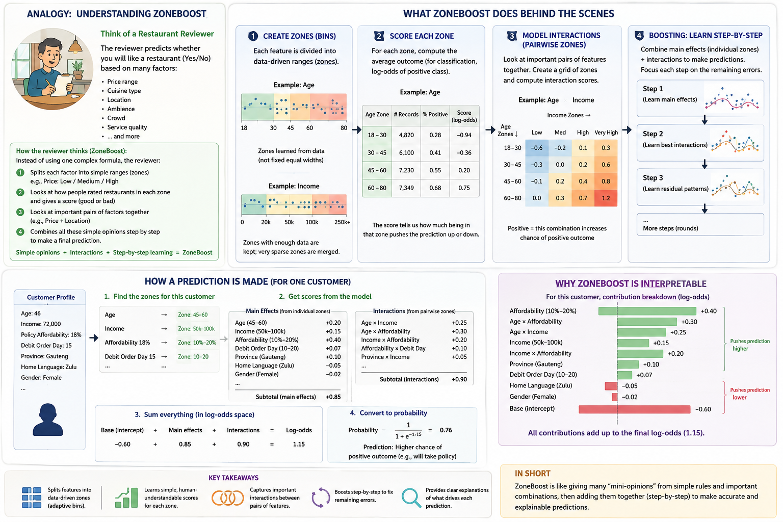
No decision trees, no gradient descent, no neural weights — just zones and averages, boosted.
The Weak Learner
Each boosting round fits a weak learner made of two transparent pieces, both built by splitting each predictor's axis into a small number of data-driven zones and averaging the current residual within each zone (or zone pair).
Main Effects
For each predictor, a 1D lookup from zone to average residual — the simplest possible model of "what does this variable alone tell us about the current error."
Interactions
For every pair of predictors, a 2D lookup from their joint zones to average residual, capturing effects neither variable explains alone. An interaction's contribution is never split back between its two variables — it's reported and explained as its own term (see Explaining Predictions).
Empirical Bayes Shrinkage
Every zone's own mean is shrunk toward a hierarchical prior via empirical
Bayes — so sparse zones lean toward their prior instead of overfitting a
handful of rows (see Empirical Bayes
Shrinkage below for the full mechanics). Each round's correction is applied at a
small, shrunk step (learning_rate) and added to a running prediction,
exactly like standard gradient boosting. row_subsample /
col_subsample add stochastic-gradient-boosting-style regularization by
fitting each round on a random subsample of rows and columns.
Continuous vs. Categorical Zones
Continuous predictors get adaptive zone boundaries, found the way a regression tree finds a split — the cut that most reduces the target's within-zone variance — re-derived fresh every round from that round's residual, rather than fixed quantile bins computed once.
Categorical predictors (declared via categorical_features,
or auto-detected from object/category/bool
dtype) skip that search entirely: every distinct value gets its own zone. A cut-point
search assumes two values that are numerically close behave alike — true for a
continuous variable, false for a nominal category like a neighborhood ID, where
there's no reason two adjacent label-encoded values behave similarly.
categorical_features rather than
raising max_zones. Raising the continuous cap for everyone gives every
continuous variable more per-round fitting flexibility, which in practice mostly
helps it overfit noise rather than capture real structure.
Missing Values
Both continuous and categorical columns accept NaN/None directly — no imputation needed beforehand. A missing value gets its own dedicated zone, kept separate from an unseen-but-real category (a value that exists but wasn't present at fit time), the same way an unseen category is handled. If missingness itself is informative (a common, real phenomenon — e.g. a sensor reading that's absent exactly when it would have been extreme), the model learns that: the missing zone gets its own data-driven average contribution from whichever training rows were actually missing for that column, rather than being silently imputed away or corrupting the adaptive split search for the column's present values.
From Regression to Classification
ZoneBoostClassifier uses the identical weak learner — same
main effects, same interactions, same empirical-Bayes shrinkage. The only change is where
boosting happens: each round is fit against the residual in log-odds
space (y - sigmoid(current_score), the standard logistic-loss
gradient) instead of the raw target, and predictions are squashed through a sigmoid at
the end. This is the standard way gradient boosting generalizes from regression to
classification.
Binary targets fit a single log-odds booster — already a principled, single sigmoid with no heuristic involved. 3+ classes use native multinomial (softmax) boosting (see "Native Multinomial Boosting" below): one booster maintains all K classes' logits jointly and optimizes the true softmax cross-entropy, rather than K independent one-vs-rest boosters normalized together after the fact.
Adaptive Interaction Order
By default zoneboost learns main effects and every pairwise interaction
(max_interaction_order=2). Setting max_interaction_order=3
additionally attempts a bounded, adaptive search for 3-way interactions each round:
- Main effects and pairwise interactions are fit exactly as always.
- Candidate triples are seeded from the columns appearing in that round's
strongest pairs — not every possible
(a, b, c)triple, which would be combinatorially expensive for datasets with many predictors. - Each candidate is checked against what main effects and its three constituent pairwise interactions would already predict. Only if a joint 3-way zone grouping still explains meaningful residual variance beyond that — evidence of a genuine higher-order pattern, not something pairwise terms already cover — does it clear the bar.
- Surviving candidates are ranked by that evidence, and only the strongest
max_triple_interactionsare kept per round.
If nothing clears the bar in a given round, no triples are added that round — this
is why the default (max_interaction_order=2) produces identical models to
every prior release: the 3-way search is strictly opt-in.
| Parameter | Default | Description |
|---|---|---|
max_interaction_order | 2 | Set to 3 to enable the 3-way search above. |
max_triple_interactions | 5 | Cap on how many 3-way terms a single round may add. |
triple_min_gain | 0.05 | How much residual-explained evidence, relative to a candidate's strongest constituent pair, is required to accept it. |
A 3-way term shows up in explain() output
exactly like a pairwise one, just with three predictor names joined by
" x " — e.g. "price x location x season" — and its
contribution still sums exactly into the prediction alongside every other term.
Cross-Fitted Cell Means
Every zone's mean (main effect, pairwise, or 3-way) is otherwise computed from the
same rows a round then scores — each row's own residual partly determines the zone
mean it's then judged against, the same in-sample leakage CatBoost's ordered boosting
was built to fix. Left alone, this biases the boosting trajectory optimistic about
sparse zones (small min_zone_frac continuous zones, high-cardinality
categoricals), since a zone with a handful of rows can end up mostly reconstructing
its own members' values rather than reflecting real structure.
Each round instead splits its (already row/column-subsampled) rows into
cross_fit_folds folds (default 5) and scores each fold only with zone
tables built from the other folds — no row is ever scored with a table that
included its own value. Only the training signal is affected; the tables actually
stored in rounds_ and used by predict/explain
still use every available row, since new data was never part of the leakage to begin
with. This is on by default, not a max_interaction_order-style opt-in —
it's a correctness fix, not a feature.
raw's spread to match the residual's regardless of how well the two
actually correlate — harmless when raw is in-sample-inflated (as it
always was pre-cross-fitting), but once cross-fitting honestly reveals a round found
no real signal, raw's variance can legitimately collapse toward zero,
and dividing by a near-zero value amplifies noise instead of correctly damping it.
This was first fixed with an ordinary-least-squares rescale, later superseded by the
Lasso fit described in Lasso Stacking below (same
non-amplifying property, plus per-term weights instead of one shared scale).
| Parameter | Default | Description |
|---|---|---|
cross_fit_folds | 5 | Number of folds used to compute each round's training signal honestly. Falls back to no cross-fitting if a round's row count is smaller than 2 folds. |
Empirical Bayes Shrinkage
Every prior release weighted a zone's contribution by
confidence = counts / counts.max() — a flat, ad hoc discount relative to
that round's busiest zone. This is replaced by an empirical-Bayes
(m-estimate) shrinkage of the zone's mean itself:
shrunk_mean = (n * cell_mean + m * prior) / (n + m)A zone needs about m rows of its own (shrinkage_m,
default 10) before it's trusted as much as its prior; fewer rows lean toward the
prior, more rows lean toward its own data. Critically, the prior is
hierarchical, not the flat global mean:
- Main effects shrink toward the global mean.
- Pairwise interactions shrink toward the additive combination of their own row and column marginals (each already shrunk the same way) — for a sparse joint cell, "what row A's zone alone predicts, plus what column B's zone alone predicts" is a far better guess than the overall average of everything.
- 3-way interactions shrink one level deeper still, toward the additive combination of their three main effects and three pairwise interactions (all already shrunk).
This fully replaces the confidence mechanism rather than supplementing it — once a
cell's own mean is properly shrunk in proportion to how little data supports it, a
separate trust-discount multiplied on top is redundant. Like the cross-fitting fix,
this is on by default: a more principled estimate, not a
max_interaction_order-style opt-in.
| Parameter | Default | Description |
|---|---|---|
shrinkage_m | 10.0 | Empirical-Bayes shrinkage strength — a zone needs about this many rows of its own before it's trusted as much as its (hierarchical) prior. |
Learning shrinkage_m instead of hand-setting it.
shrinkage_m plays the role of sigma² / tau² in
the normal-normal hierarchical model this shrinkage formula already implies
(sigma² = within-zone/sampling variance, tau² =
between-zone variance of the true zone effects) — a well-known equivalence
(Efron & Morris), the same "compound normal means" problem DerSimonian &
Laird solve for random-effects meta-analysis variance components.
learn_shrinkage_m=True estimates this separately for main effects and
for pairs each round (pooling raw zone/cell statistics across every column or pair
fit at that level), via the DerSimonian-Laird method-of-moments estimator — chosen
over a full numerical marginal-likelihood search for being closed-form and cheap
enough to run every round without becoming the new bottleneck.
model = ZoneBoostRegressor(learn_shrinkage_m=True).fit(X, y)
model.rounds_[0]["diagnostics"]["learned_shrinkage_m"] # {"main": ..., "pair": ...}shrinkage_m constant (deferred: the adaptive-triple-selection
accept/reject gain test already uses m to decide which
triples survive, before the accepted set is known, making a triple-level estimate
circular in a way mains/pairs aren't). Falls back to shrinkage_m
itself whenever there isn't enough evidence to estimate anything better (a single
zone, or no detectable signal beyond sampling noise).
x1² main effect and a comparatively sparser
0.3·x1·x2 interaction, the learned shrinkage strength
averaged 39.7 for main effects versus 103.0 for
pairs across 80 rounds — pairs earned heavier shrinkage than mains in
78.8% of rounds, exactly the pattern sparser interaction cells
should show relative to better-supported main effects. Training RMSE was
essentially a wash against the hand-set default (1.0076 learned vs.
1.0071 at m=10) — the value here is a principled,
per-level calibration that removes a hand-tuned constant, not a guaranteed
accuracy improvement. learn_shrinkage_m=False (the default) is
bit-identical to every prior release.
Robust Cell Statistics (trim_fraction)
A handful of outlier rows landing in one zone can drag that zone's plain
bincount-summed mean toward them — nothing about a mean alone is robust
to contamination. trim_fraction swaps the raw per-zone statistic for a
trimmed mean instead: sort a zone's own rows, drop the top and
bottom trim_fraction of them, and average the rest — still a real
average of real, observed rows (no value is altered, unlike winsorizing), just fewer
of them. The identical empirical-Bayes shrinkage formula above applies to whichever
raw statistic comes out, exactly the way it already tolerates a quantile as the raw
statistic under loss="quantile".
model = ZoneBoostRegressor(trim_fraction=0.1).fit(X, y) # drop 10% from each tail, per zoneUnlike loss="quantile", this doesn't change what's being
estimated. Quantile mode targets a genuinely different point of the
conditional distribution (a location-family generalization); a trimmed mean is still
estimating the same conditional mean, just made robust to outliers — so,
unlike quantile mode, the Lasso combination step is completely unaffected
(Lasso's intercept being the residual's own mean isn't fighting the
target the way it does for a quantile-shrunk term). The two are mutually exclusive:
trim_fraction > 0 with loss="quantile" raises
ValueError at fit.
trim_fraction, the same disclosed scope
loss="quantile" already carries for those (verified directly: none of
_pair_shrunk_deviation/_triple_shrunk_deviation/
_fit_pairs/_select_triples even accept a
trim_fraction parameter). Compatible with
"poisson"/"gamma"/"tweedie" — each round's
own main-effect zone statistics are robustified there too — but the
initial baseline intercept for those three losses stays
_glm_baseline's closed-form, untrimmed formula (no simple trimmed
equivalent for it). Winsorizing (clip outliers to a threshold instead of dropping
them) is a natural extension using the identical per-zone grouping logic, but isn't
shipped here — one well-tested mechanism over two half-built ones.
Measured, honestly: on synthetic data (y = 2x,
n=2000) with 5 extreme outlier rows planted in one zone (x
in [4, 5), each inflated by +200), the default
trim_fraction=0.0 predicted 17.45 at x=4.5
against a true value of 9.0 — dragged far off by the outliers.
trim_fraction=0.2 predicted 9.60, and RMSE against a
clean holdout dropped from 2.44 to 0.65.
trim_fraction=0.0 (the default) is bit-identical to every prior
release.
Sample Weighting (sample_weight)
ZoneBoostRegressor.fit(X, y, sample_weight=...) — a per-row weight,
like offset, not a tuning knob. Unlike offset, it only
affects how the model learns (zone construction, empirical-Bayes shrinkage,
GLM baseline/deviance, the Lasso/QuantileRegressor combination step) —
never what a fitted model predicts for a given input, so there is no
corresponding predict(X, sample_weight=...).
The empirical-Bayes shrinkage formula itself needs zero changes to
support this: (counts * cell_stat + m * overall_stat) / (counts + m) is
pure arithmetic on whatever counts/cell_stat are — making
counts a weighted sum and cell_stat a
weighted mean instead of a row count/plain mean is enough, since
m already means "how much evidence before trusted as much as the prior,"
which composes correctly whether that evidence is measured in rows or weight.
Unlike trim_fraction (main effects only), this generalizes to
pairs and triples for free — they already route through the same weighted
_zone_raw_stat/_zone_shrunk_deviation machinery internally
for their own marginal priors and joint-cell statistic, so threading
sample_weight through those shared functions once benefits every term
order automatically.
model = ZoneBoostRegressor().fit(X, y, sample_weight=exposure)loss="quantile" or
trim_fraction > 0 (raises ValueError) — weighted
quantiles require picking one of several genuinely ambiguous conventions for
generalizing linear-interpolation quantiles to unequal weights (numpy's own
weights support for np.quantile requires switching
interpolation methods entirely, breaking bit-identical behavior even for uniform
weights), and a weighted trimmed mean has an analogous "drop by row count or by
weight mass?" ambiguity — both scoped out rather than guessed at. Compatible with
"squared_error"/"poisson"/"gamma"/
"tweedie" (all share the unambiguous, weighted-mean raw statistic).
Pair-screening's cheap ANOVA proxy and adaptive_boundary_smoothing's
own internal fitting stay unweighted regardless — the same disclosed scope other
approximations in this library already carry. Row/column subsampling stays uniform
regardless of weight. predict_interval's conformal calibration is not
weighted — weighted conformal prediction is a distinct research problem, not
attempted here. Weights must be non-negative; a zero weight is valid.
Measured, honestly: on the identical outlier scenario as
trim_fraction above, giving the 5 outlier rows
sample_weight=0.001 instead of dropping them recovered a prediction of
9.07 at x=4.5 (true value 9.0) versus 17.45
unweighted. On a genuine a×b interaction with 8 joint-cell outliers,
down-weighting them moved the predicted joint effect from 3.52 to
2.75 (true value 2.70) — confirming pairs really do inherit the
weighting, not just main effects. sample_weight=None (the default) is
bit-identical to every prior release — including a subtle case caught during
development: the min_zone_frac/min_zone_abs zone-size guards
must floor to the same integer row count as the unweighted path even when a
sample_weight array of all-ones is passed explicitly, or "uniform weight"
would silently stop being bit-identical to "no weight."
Lasso Stacking
Every prior release combined a round's terms by averaging every contribution
equally (raw = contributions.mean(axis=1)), then fit one shared scale for
the whole blend — every term got the same diluted 1/n_terms weight
regardless of relevance. This is replaced by a Lasso fit that treats
each term's own (cross-fitted) contribution as its own feature:
- An irrelevant term's weight gets zeroed by the L1 penalty.
- A strong term gets its own learned weight instead of a diluted share.
- The fitted weights are themselves a real interaction-importance ranking, flowing straight through feature_importance() / explain() with no new API needed.
Both sides are standardized before fitting (each contribution by its own std, the
residual by its own) so stacking_alpha — the L1 regularization strength —
is unitless and comparable across rounds and datasets.
| Parameter | Default | Description |
|---|---|---|
stacking_alpha | 0.01 | Lasso regularization strength for combining a round's terms, in the standardized space described above. |
Soft Zone Boundaries
Continuous zone boundaries were hard cuts: a value one unit below a cut point and one unit above it land in completely different zones with independently-shrunk means — a "cliff edge" discontinuity in the prediction at the exact boundary, which doesn't match how a genuinely continuous relationship should behave. Every real zone now also gets a centroid — the empirical mean training-x-value of the rows that landed in it — and a lookup blends between a value's own zone and whichever neighboring zone its centroid points toward, rather than hard-assigning it to exactly one:
- 0 exactly at its own zone's centroid, 1 exactly at the neighbor's, linear between, clamped past either end (leftmost/rightmost zone, or a single-zone column) so it never reaches past a non-existent neighbor.
- Main effects become a 2-point linear blend; pairwise interactions become the standard 4-corner bilinear blend; triples become the 8-corner trilinear analog.
- Categorical columns and missing values are an exact no-op (always fully their own hard zone) — there's no meaningful "distance" to interpolate along a nominal category. A pair/triple with a categorical member naturally interpolates only along its continuous member(s).
Zone construction (the adaptive split search, min_zone_frac,
max_zones) and each zone's own fitted mean (still computed by
hard-grouping training rows, unchanged) are untouched — only how a value is
looked up against an already-fitted grid changes.
Cyclic Backfitting
A pairwise interaction's shrunk deviation was the joint cell
mean — not an interaction-only signal. If column a has a genuine main
effect and no real interaction with b exists, the joint (a,
b) cell mean still reflects a's main effect (shrunk toward a
dev_a + dev_b prior that itself contains it), so the stored pair
redundantly re-encodes signal a's own main effect already captures —
and since Lasso stacking can only apply one scalar weight per term, it can't
cleanly cancel a redundant shape baked in cell-by-cell. The same gap
applied to triples: the accepted triple's stored value was fit against the raw
residual, even though the accept/reject gain test already computes an approximate
"residual after lower-order terms" for its own threshold decision.
Terms are now fit via a single backfitting pass each round — main effects first, then pairs (backfit against their own two main effects), then triples (backfit against their own three main effects, with pairs handled automatically inside the triple's own recursive prior computation) — so a pair's or triple's stored value is genuinely interaction-only rather than a partial copy of what a lower-order term already explains. Not a full iterate-to-convergence GAM backfit: one ordered pass per round, relying on the boosting loop's own many rounds for further refinement over time.
explain()/feature_importance()
show, not just internal accuracy. Like the four changes above, this is on by
default; there's no tunable knob to expose, so no new parameter was added.
Monotonic Constraints
Unlike the four changes above, this one is opt-in: it encodes
domain knowledge the model has no way to infer on its own (e.g. "take-up must not
decrease as affordability rises"), rather than a general correctness or estimation
improvement everyone should get by default. Pass
monotonic_constraints={"column": +1} (non-decreasing) or
{"column": -1} (non-increasing) — same name/index convention as
categorical_features — and that column's own main effect
is projected onto the nearest monotonic sequence across its zones via a
row-count-weighted isotonic regression, applied after empirical Bayes shrinkage so
sparse zones don't distort the projection.
- Inherited by interactions. Every pairwise/triple term the column participates in is also projected along that column's own axis, holding the other axis/axes fixed — automatic whenever a constraint is declared, no separate opt-in. See "Global Shape Constraints" below for how.
- A continuous column's zones are already ordered low → high by construction, so there's no threshold or window to tune — just a direction.
- A constraint declared on a categorical column is silently dropped (no meaningful
order to constrain for a nominal category) rather than raising; an invalid direction
(anything other than
-1/1) does raise, atfit()time. - The missing-value zone is excluded from the projection — it's a separate bucket, not part of the ordered continuum.
monotonic_constraints=None (the default) reproduces the exact
same predictions as before this change — verified bit-for-bit.
Pair Screening
Every round fits every C(p, 2) pairwise interaction
among that round's (subsampled) predictors — fine for a modest number of columns, but
two costs scale with pair count: cross-fitting recomputes every pair once per fold (a
straight cross_fit_folds× multiplier), and Lasso stacking fits one feature
per term, so hundreds/thousands of pairs make the per-round Lasso fit itself the
bottleneck. Like monotonic constraints, this is opt-in — dropping weak
pairs entirely changes results (some would have gotten a small nonzero Lasso weight),
so it's a genuine approximation tradeoff, not a free correctness fix.
max_pair_interactions caps how many pairs a round keeps via
cheap-then-exact hierarchical discovery, rather than fitting every
pair in full and ranking afterward: every candidate pair is scored with a fast,
single-pass ANOVA-style interaction statistic (does the joint cell mean deviate from
what the two marginals alone would predict) on an honest, cross-fitted
main-effects-only residual — never the same in-sample residual a pair will later be
fit against — and only the top-scoring pairs (plus whatever pairs the 3-way
interaction search needs for its own candidate columns, when
max_interaction_order=3) ever pay the full empirical-Bayes fitting cost.
Applied before the expensive fit rather than after, so
_select_triples still finds genuine 3-way interactions even when only
one pair survives into the final model — its own candidate-column search runs on the
cheap score, computed for every pair, not just the kept ones.
O(p²)
Python-loop overhead itself, which both the old and new mechanism pay equally. The
net result is a real but modest ~1.4x speedup, consistent from 80
to 300 columns, not an order-of-magnitude win. Leaving
max_pair_interactions=None (the default) keeps every pair — the exact
same behavior as before this change, verified bit-for-bit.
scipy.sparse) version came out consistently slower than the
plain loop (0.2x–0.5x): sparse-sparse matmul on a one-hot indicator matrix still
pays for every (row, zone_a, zone_b) triple regardless of how sparse
the output is, so it does the same O(n_rows·p²) work with more
overhead, not less. Switching to a dense BLAS matmul recovered a real speedup
(~1.4x–1.8x), but only for wide, fairly shallow data (reliable from
roughly 80–120+ columns at a few thousand rows); at more rows per column it
measured up to ~3x slower, since building the dense matrix and its
full cross-product has a fixed cost that doesn't always pay off. There's no cheap,
reliable way to predict which side of that crossover a given fit lands on without
risking a real regression for some users — so it isn't wired into the default
screening path. The function (_batched_pair_scores) ships anyway,
tested and exact, for advanced callers who've benchmarked their own workload and
know it's wide-and-shallow enough to benefit.
Hierarchical Zones (Grouped Data)
Grouped data — patients within hospitals, customers within regions — wants
partial pooling: a group with few rows of its own should lean on the overall
pattern, a group with many rows should be trusted on its own terms. This already
happens automatically whenever two columns are fit as a pairwise interaction: the
joint (zone A, zone B) cell shrinks toward overall + column A's own marginal
deviation + column B's own marginal deviation (see Empirical Bayes Shrinkage above) — local
(joint cell) ← regional (each column's own marginal effect) ← global
(overall mean), with no new math required.
group_col="hospital" (a column name or index) turns that into a
guarantee rather than a coincidence: the group column is never
dropped by col_subsample, and every (feature, group_col)
pair is never dropped by max_pair_interactions screening (an explicit
forbidden_interactions entry still wins). Nothing else changes —
explain(X) already reports both halves of the decomposition directly:
the income column is the pooled, regional/global effect;
"income x hospital" is the local deviation one specific
hospital adds on top of it.
model = ZoneBoostRegressor(group_col="hospital").fit(X, y)
contrib = model.explain(X)
contrib["income"]              # regional/global-pooled income effect
contrib["income x hospital"]   # this row's own hospital's local deviation
Every existing reliability/evidence mechanism extends to group_col
for free, since it's an ordinary pairwise interaction under the hood:
track_reliability=True + explain(X, include_reliability=True)
reports support/shrinkage_fraction for the
"income x hospital" term exactly like any other, and
evidence_report(X) folds it into its per-row evidence_score.
"income x hospital" cell came back with support≈2.9 and
shrinkage_fraction≈0.79 (79% weight on the hierarchical prior) versus
support≈188 and shrinkage_fraction≈0.075 (~7.5%) for the
two large hospitals — and evidence_report's evidence_score
for the tiny hospital's rows was 0.13
(pct_contribution_from_sparse_cells≈0.73) versus 0.5 for
the large hospitals', all read directly off existing, unmodified reporting — no new
methods were needed for any of this.
shrinkage_m
rather than a dedicated group-level shrinkage constant. Regressor only. All
deferred, disclosed. Leaving group_col=None (the default) reproduces
the exact same predictions as if this parameter didn't exist.
Native Multinomial Boosting
3+ class problems previously used one-vs-rest: K completely independent log-odds boosters, each fit against its own binary sigmoid residual, then normalized to sum to 1 at predict time. Each class's booster never knew about the other K-1 classes' current scores — a reasonable, standard heuristic, but not what genuinely optimizing multinomial cross-entropy looks like. This is now on by default — one-vs-rest was never a deliberate permanent design choice. Binary classification (already a single principled sigmoid, no one-vs-rest heuristic involved) is completely unaffected — verified bit-for-bit.
A single booster now maintains all K logits jointly per row. Each round,
p = softmax(scores) and every class k's residual is
1(y==k) - p[:, k] — the true joint gradient, where raising one
class's score correctly lowers every other class's probability through the
shared softmax denominator. A separate weak learner is still fit per class per
round (the same weak_learner_fit reused unchanged, just called K
times against K different residuals), then the K raw outputs are
centered to sum to zero per row before being added to the
running scores. This centering is mathematically a no-op for predictions —
softmax is shift-invariant to any constant added equally to every class's
logit — it exists purely so each class's own contribution is uniquely
defined rather than ambiguous up to an arbitrary shared function, which
matters specifically because explain()'s per-class attribution
needs to be unique to mean anything.
explain() reflects this: each class's DataFrame gains one
extra column, "_softmax_centering" — the cumulative version of
that same per-round centering, identical across every class. With it
included, softmax(explain(X)[classes_[0]].sum(axis=1), ...)
reproduces predict_proba(X) exactly (verified to machine
precision). calibrate=True still works for multiclass: one
isotonic calibrator per class, calibrating that class's own marginal softmax
probability, renormalized back to sum to 1 afterward.
| Metric | One-vs-rest (old) | Native softmax (new) |
|---|---|---|
| Accuracy | 0.958 | 0.962 |
| Log-loss | 0.289 | 0.202 |
| Minority-class reliability error | 0.041 | 0.030 |
Breaking change, disclosed:
boosters_
(previously a {class_label: booster} dict for 3+ classes) is
replaced by a single softmax_booster_ attribute. Any code
inspecting boosters_ directly for a multiclass model needs to
update to softmax_booster_.
Prediction Intervals (Regressor)
ZoneBoostRegressor.predict_interval(X, alpha=0.1) returns a
constant-width (lower, upper) band around predict(X) via
split conformal prediction — a distribution-free marginal coverage
guarantee, P(y in interval) >= 1 - alpha, assuming exchangeability
(Vovk / Lei et al.'s standard split-conformal setup), not a heteroscedasticity-aware
or locally-adaptive variant. The margin is the finite-sample-corrected
ceil((n+1)*(1-alpha))-th smallest absolute residual measured on a
genuinely held-out split — never training rows. Purely additive: every existing
method's output is unaffected. Requires validation_fraction > 0 or
calibration_fraction > 0 (see "Honest Data Splits" below); raises
ValueError otherwise.
alpha=0.1 achieved ~90.2% empirical
coverage on held-out data.
Mondrian (group-conditional) coverage: a single global margin
gives distribution-free marginal coverage — but if a minority segment
behaves systematically differently (different residual variance, a different
regime), its own coverage can sit well below the target even while the marginal
number looks fine. mondrian_col="region" at fit time
stratifies the calibration-split nonconformity scores by that column's own values,
so predict_interval gives each row its own group's margin instead of
one global margin for everyone — reusing the exact same calibration split already
computed, no new held-out data needed. Independent of group_col
(different purpose: calibration stratification vs. hierarchical partial pooling in
the boosting model itself) — set one, both, or neither.
model = ZoneBoostRegressor(mondrian_col="region").fit(X, y)
model.predict_interval(X)  # each row's margin comes from its own region
A group with fewer than mondrian_min_group_size (default
20) calibration rows falls back to the global margin (a per-group
quantile from too few scores is unstable) — so does an unseen group value at
predict_interval time.
mondrian_col set, the minority segment's own coverage rose to
87.7%, with overall and majority coverage still close to the
90% target (89.6%/89.8%) — reproducing exactly the "marginal 90% can hide 70% on
a minority segment" problem this fixes. mondrian_col=None (the
default) is bit-identical to every prior release.
Probability Calibration (Classifier)
ZoneBoostClassifier(calibrate=True) recalibrates each booster's raw
probability with an isotonic regression fit on a genuinely held-out
split — the same recipe
sklearn.calibration.CalibratedClassifierCV(method="isotonic") uses, so
predicted probabilities better match empirical frequencies. Binary: one calibrator
on booster_. Multiclass: one per class on softmax_booster_,
calibrating that class's own marginal softmax probability, renormalized back to
sum to 1 afterward. Requires validation_fraction > 0 or
calibration_fraction > 0; raises ValueError at
fit otherwise. Only affects predict_proba —
explain()/feature_importance() still decompose the raw
log-odds score unchanged.
calibrate=False reproduces today's exact predict_proba
output, verified bit-for-bit) and is the only parameter that differs between the
two estimators.
Honest Data Splits (Calibration & Final Refit)
Both calibration mechanisms above originally reused the same
validation_fraction split that also drives early stopping — a disclosed
tradeoff (the round count predict uses was itself chosen to minimize
error on this exact set, which can understate the true calibration margin slightly).
Two new parameters, shared by both estimators, fix this properly:
calibration_fraction(default0.0) carves out a third, genuinely separate partition purely for calibration — never seen by either the fit split or the validation split.0.0reproduces every prior release's behavior exactly (calibration reuses the validation split, verified bit-for-bit); setting it removes the disclosed tradeoff above entirely.refit_on_full_data(defaultFalse) — oncebest_n_rounds_is chosen from the validation split, optionally retrains the deployed model on fit+validation data combined, so validation data isn't permanently withheld from the model that actually predicts.train_rmse_/val_rmse_still reflect the original selection-phase curves, not the refit pass. Requirescalibration_fraction > 0: folding the validation split into training means it can no longer double as a calibration set too, so a genuinely separate one is required (raisesValueErrorotherwise) — the one real correctness constraint that keeps the two features from silently interacting badly.
Adaptive Boundary Continuity
Soft zone boundaries made every continuous column's zone lookup unconditionally interpolate between neighboring zones — eliminating the cliff-edge discontinuity that hard zone assignment produced, but at the cost of blurring a genuinely sharp threshold just as much as a genuinely smooth relationship. A column with a real step (a policy cutoff, a regulatory cliff) has no way to tell the model "don't smooth me."
adaptive_boundary_smoothing=True (opt-in, default False)
learns one mixing weight λ per continuous column per round —
0 fully hard, 1 fully smooth — instead of always using
1. Estimated honestly, out of fold: reusing the same cross-fitting
split every round already builds, each fold's zone means are refit from the
other folds only, then scored on the held-out fold both ways (hard lookup
vs. full-smooth interpolation) against the true residual. λ is the
fraction of held-out error reduction smooth interpolation earns over hard lookup
— 1 when smooth wins clearly, 0 when hard wins clearly —
then shrunk toward 1 (the smoothness prior) via the same
empirical-Bayes pattern used everywhere else in zoneboost, governed by
boundary_shrinkage_m (default 10.0): a boundary with few
held-out rows near it leans back toward full smoothness by construction, rather
than overreacting to a handful of noisy points.
λ isn't guaranteed to sit near 1 just
because the true relationship is continuous; it sits near whichever side
actually reduces held-out error.
Measured, honestly, on a synthetic step function (true jump
of 5.0): the largest single-step prediction change across the true boundary was
0.36 with the always-smooth default, vs. 3.86 with
adaptive_boundary_smoothing=True — much closer to the real step, not
blurred away. On a genuinely curved (quadratic) relationship with few zones, RMSE
improved from 0.90 to 0.29 — the mechanism found real approximation error
interpolation could fix and leaned into it, rather than defaulting to hard lookup
out of caution. explain(X) still sums exactly to predict(X)
with the feature active (verified to float precision) — no new call sites bypass
the shared, now λ-scaled, blend.
Leaving adaptive_boundary_smoothing=False (the default) reproduces
the exact prior behavior — verified bit-for-bit. This is opt-in because the
estimate is a cross-fitted heuristic rather than a rigorous statistical test, and
it adds real per-round cost, matching the precedent set by monotonic constraints
and pair screening.
Quantile Regression
Every prior release targets the conditional mean
(loss="squared_error", the default) — a single number, no sense of
spread. ZoneBoostRegressor(loss="quantile", quantile=0.9) instead
targets a single conditional quantile of y: every
zone's fitted value becomes a shrunk quantile of the residual at that
level rather than a shrunk mean (the same (n * raw + m * prior) / (n +
m) empirical-Bayes shrinkage pattern used everywhere else in zoneboost,
applied to a quantile instead of a mean). Fit several instances at different
levels (e.g. 0.05, 0.5, 0.95) to get a full
conditional distribution.
The raw residual still drives zone-split search, cross-fitting, and pair
screening's cheap proxy identically regardless of loss (a disclosed
approximation — those stay squared-error-flavored). The round's
term-combination step, however, must change: combining
quantile-shrunk terms via an ordinary (squared-error) Lasso would silently
re-center every round's output back toward the mean/median, actively destroying
the quantile target rather than merely approximating it — confirmed empirically
during development (coverage drifted from ~90% down to ~50% over 100 rounds
before this was fixed). loss="quantile" instead combines terms via
sklearn.linear_model.QuantileRegressor (pinball loss + L1 penalty),
so the combination step stays consistent with the same loss every term's own
value was fit against.
Measured, honestly: on synthetic heteroscedastic data (noise
scale growing with x), ZoneBoostRegressor(loss="quantile",
quantile=0.9) achieved 89.4% held-out coverage below its predictions
(target 90%). QuantileRegressor's linear-programming solver is
substantially more expensive per round than the default Lasso —
roughly 30x slower end-to-end in one benchmark — a real, disclosed cost of
loss="quantile", not a free option. loss="squared_error"
(the default) is completely unaffected — verified bit-for-bit.
predict_interval raises ValueError when
loss="quantile": a constant-width margin around a single quantile
isn't a meaningful coverage interval the same way it is around a mean — see
Conformalized Quantile Regression below instead.
Not to be confused with trim_fraction (see
Robust Cell Statistics above): quantile mode
changes what's estimated (a different order statistic of y);
trim_fraction keeps estimating the mean but makes it robust to outlier
rows, so — unlike quantile mode — the Lasso combination step is unaffected. The two
are mutually exclusive.
Actuarial Losses (Poisson, Gamma, Tweedie)
loss="poisson"/"gamma"/"tweedie" target the
conditional mean of a right-skewed, non-negative target under a log
link — the frequency/severity/pure-premium pattern actuarial GLM stacks
use — boosted in link space exactly the way
ZoneBoostClassifier already boosts in log-odds space: a running
link-scale score accumulates round to round, each round's residual is the
negative deviance gradient (mu**(1 - power) * (y - mu), unifying all
three losses via the Tweedie variance power — power=1 for Poisson,
power=2 for Gamma, power=tweedie_power — default
1.5 — otherwise), stacked with the same ordinary Lasso every other
loss uses (the residual is still just a plain number to regress, no new
combination step needed), and the log link (mu = exp(score)) is
applied only once, at predict time. explain(X)
therefore sums to the link-scale score, not the final mean —
the identical convention already documented for the classifier's log-odds.
model = ZoneBoostRegressor(loss="poisson").fit(X, claims, offset=np.log(exposure))
model.predict(X, offset=np.log(exposure))          # claims per policy, exposure-adjusted
model.explain(X).sum(axis=1) + np.log(exposure)    # == log(predict(X)), exactly
offset (only meaningful for these three losses) is a per-row,
already-link-scale term — e.g. np.log(exposure), not
exposure itself — added to the model's own score before the inverse
link, the same base_margin/init_score convention
XGBoost/LightGBM use. It must be supplied again at
predict/predict_interval time for new data (the model
never learns it); omitting it defaults to 0 everywhere.
train_rmse_/val_rmse_ store the corresponding mean
deviance (sklearn.metrics.mean_poisson_deviance/
mean_gamma_deviance/mean_tweedie_deviance) rather than
RMSE for these three losses. Zone construction, cross-fitting, and pair
screening's cheap proxy stay squared-error-flavored on the link-scale residual
regardless — the same disclosed approximation loss="quantile"
already uses. Requires y >= 0 for
"poisson"/"tweedie", y > 0 for
"gamma" — raises ValueError at fit
otherwise. predict_interval is not available for these three losses
(a constant-width additive margin isn't a sensible interval for a skewed,
non-negative target).
sample_weight is not yet
supported for any loss (a separate, larger change to the empirical-Bayes
shrinkage machinery itself — _zone_raw_stat and everything built
on it currently compute unweighted row counts). tweedie_power is a
fixed, user-set constant, not auto-tuned.
Measured, honestly: on synthetic insurance-style frequency
data (age + region effects, exposure ranging 0.1-1.0 policy-years), a Poisson
model with offset=log(exposure) achieved a mean deviance of
0.626 versus 0.695 for a naive constant-rate baseline
(same total claims, no covariates) — a real 9.9% reduction. On
synthetic severity data, a Gamma model reduced mean deviance from
0.473 (constant-mean baseline) to 0.433, an
8.5% reduction. loss="squared_error"/
"quantile" are completely unaffected — verified bit-for-bit against
the prior release.
Zone-Native Survival Analysis
Piecewise-exponential hazard models — the standard actuarial/biostat
approach to time-to-event data — reduce exactly to the Poisson-with-
offset machinery above: split follow-up time into intervals, expand each
subject into one row per interval reached (covariates, whether the event
happened in that interval, how much exposure time it contributed), and a
plain loss="poisson" fit on that expanded table is the
hazard model — no new boosting mechanism.
zoneboost.ZoneBoostSurvival does exactly this expansion
internally, wrapping one ZoneBoostRegressor.
from zoneboost import ZoneBoostSurvival

model = ZoneBoostSurvival(n_intervals=10).fit(X, duration, event)
model.predict_survival_function(X)      # S(t) per row, per query time
model.predict_cumulative_hazard(X)      # H(t) per row, per query time
model.regressor_.explain(X_expanded)    # transparent hazard decomposition
Interval boundaries default to quantiles of the observed event
times (event-dense intervals), with the last interval always open-ended so
every subject's tail risk is covered. The fitted rate at offset=0
for any (covariates, interval) combination is exactly the hazard — the same
mu = exp(link_pred + offset) identity the actuarial losses use,
just with offset set to zero instead of a real exposure term.
This gives a genuine, structural difference from Cox proportional
hazards, not just a reframing: the baseline hazard is an ordinary
main effect over an interval-start column, fit by zoneboost's own
adaptive continuous zoning — no assumed parametric shape, unlike Cox's
implicit "same shape for everyone" baseline. And whenever the underlying
estimator's max_interaction_order=2, a covariate can interact
with that interval-start column — a time-varying effect, the exact
assumption Cox proportional hazards rules out by construction. Because it's
still just a ZoneBoostRegressor fit, explain()
decomposes any subject's log-hazard into baseline-time shape + covariate
main effects + interactions, fully transparent — not a post-hoc
approximation of a black-box partial likelihood.
duration=0), no interval censoring, no competing risks;
event is a plain 0/1 indicator. Covariates are time-invariant:
X is one row per subject at baseline, and can't change value
mid-follow-up in this pass. sample_weight isn't supported,
consistent with every other GLM loss. Ties in duration need
no special handling — a genuine advantage of the piecewise-exponential
reduction over Cox's partial-likelihood tie-breaking machinery, worth
noting as a real plus, not just a limitation elsewhere.
Measured, honestly: on synthetic data with a real
age-dependent hazard (n=3000, ~39% events observed), a
ZoneBoostSurvival fit achieved a concordance index of
0.652 on training data, versus exactly
0.500 (chance) for the same model fit with the covariate
zeroed out — confirming the model genuinely uses the covariate signal
rather than just fitting the baseline hazard shape.
predict_survival_function was verified non-increasing in
t for every row, and predict_cumulative_hazard
non-negative and non-decreasing, on every test dataset tried.
Conformalized Quantile Regression (CQR)
Split-conformal prediction intervals give a
distribution-free coverage guarantee, but the margin is a single fixed width
added to every row — it can't narrow where the model is confident or widen where
y's true spread is genuinely larger. ConformalizedQuantileRegressor
fixes this by conformalizing a quantile band instead of a
mean:
from zoneboost import ConformalizedQuantileRegressor

cqr = ConformalizedQuantileRegressor(alpha=0.1, random_state=0).fit(X, y)
lower, upper = cqr.predict_interval(X)
Internally, two ZoneBoostRegressor(loss="quantile", ...) models
are fit at levels alpha/2 and 1 - alpha/2 (the raw
quantile band), on its own train split. On a third, genuinely
held-out calibration split (never seen by either quantile model's own training),
the CQR nonconformity score E_i = max(q_lo(X_i) - y_i, y_i -
q_hi(X_i)) is computed per row, and the same fixed additive margin (the
finite-sample-corrected quantile of these scores — the identical formula
predict_interval itself uses) is added to both quantile predictions.
This still gives the exact same distribution-free marginal coverage guarantee as
split-conformal (P(y in interval) >= 1 - alpha, under
exchangeability) — but because the quantile predictions themselves already vary
with X, so does the total interval width, unlike a plain
split-conformal band's single constant-width margin.
Measured, honestly, on the same synthetic heteroscedastic
dataset as above: ConformalizedQuantileRegressor(alpha=0.1) achieved
88.7% held-out coverage (target 90%), with mean interval width
3.13 in the low-variance region (x < 2) versus
12.70 in the high-variance region (x > 8) —
genuinely adapting to X, roughly 4x wider where y's true
spread actually is larger. For contrast, ZoneBoostRegressor.predict_interval
on the identical data achieved 88.0% coverage with a constant 7.97
width in both regions, by construction — too narrow where variance is
high, too wide where it's low.
estimator (default None → a plain
ZoneBoostRegressor()) is an unfit template supplying every tuning
knob other than loss/quantile/
calibration_fraction/random_state (which this class
always manages itself) — the same meta-estimator pattern sklearn itself uses
(e.g. CalibratedClassifierCV(estimator=...)), rather than
duplicating dozens of ZoneBoostRegressor parameters onto this class.
Not a RegressorMixin — there is no meaningful single-point
predict, only predict_interval.
Non-crossing rearrangement: lo_/hi_
are two independently-fit models, so nothing guarantees
lo_.predict(x) <= hi_.predict(x) for every row ("crossing"). Both
are rearranged (Chernozhukov, Fernandez-Val & Galichon, 2010) — for exactly
two quantile levels, an elementwise min/max swap —
before computing calibration scores and before returning an interval,
unconditionally rather than behind a parameter: rearrangement never increases
estimation risk, and is a no-op wherever a row was already ordered, so this never
changes output on data where crossing didn't occur (verified directly, not just
argued).
Global Shape Constraints
Four related mechanisms for declaring shape knowledge the model has no way to
infer on its own — all opt-in, all main-effects-focused, all reusing
the same {column: ...} declaration convention as
monotonic_constraints.
Interactions inherit monotonicity. Declaring
monotonic_constraints={"age": 1} now also projects every pairwise/triple
interaction age participates in along age's own axis
(holding the other axis/axes fixed) — via sklearn.isotonic.IsotonicRegression
fit fiber-by-fiber (one independent fit per slice along the constrained axis),
weighted by that slice's own row counts, the multi-dimensional generalization of the
main effect's own projection. Without this, a column's total dependence on
the target (main effect + every interaction it's part of) could still come out
non-monotonic overall, undermining the point of declaring the constraint in the first
place.
monotonic_constraints is declared — disclosed as completing the
feature's original intent (interactions were deliberately unconstrained before),
not a free correctness fix. A term with more than one constrained axis is projected
axis-by-axis in a fixed order — a disclosed heuristic, not a jointly-optimal
multi-dimensional isotone regression, consistent with cyclic backfitting's own
single-pass approximation.
Measured, honestly, on synthetic data with a genuine non-monotonic dip in an interaction term: the unconstrained interaction's largest single-step decrease was -0.189; constrained, it was exactly 0.000 (fully non-decreasing).
Convexity/concavity constraints:
convexity_constraints={"column": +1} (convex) or {-1}
(concave) forces a continuous column's main effect onto a convex/concave
sequence. A convex piecewise-linear function through zone centroids
(center_i, y_i) requires non-decreasing slopes
(y[i+1]-y[i])/(center[i+1]-center[i]) — not non-decreasing raw
differences, since zones are rarely evenly spaced (adaptive zone boundaries). This
isotonic-regresses those slopes, reconstructs, and re-centers to the original level.
Measured, honestly: across 60 rounds fit on genuinely non-convex (wiggly) synthetic data, every single round's own projected slopes were non-decreasing (0 violations) — the guarantee holds exactly where it's actually made.
Ensemble-Level Guarantees
strict_shape_constraints=True restricts a round's own Lasso-stacking
weight to be non-negative for every term a
monotonic_constraints/convexity_constraints entry applies to
(a monotonic column's own main effect and every pair/triple it participates
in, since interactions inherit the projection too; convexity is main-effects-only) —
turning the per-round-only guarantees above into a real ensemble-level one: a
non-negative-weighted sum of individually-monotonic (or individually-convex) round
contributions is itself monotonic (or convex), a mathematical guarantee, not a
heuristic.
model = ZoneBoostRegressor(
    monotonic_constraints={"x1": 1}, strict_shape_constraints=True,
).fit(X, y)
Implemented by representing every unconstrained term's weight as the
difference of two non-negative variables (w_free = w_free+ - w_free-)
and fitting a single sklearn.linear_model.Lasso(positive=True) on the
expanded design — Lasso only supports positive=True for
every coefficient, not a per-term subset, but at the L1-optimal solution
w_free+/w_free- are never both positive for the same term
(reducing both by min(w_free+, w_free-) leaves the fit unchanged but
strictly shrinks the penalty), so w_free+ - w_free- recovers
exactly the solution the original mixed-sign-constrained problem would have —
not an approximation, and reuses sklearn.linear_model.Lasso entirely, no
new numerical algorithm.
bounded_effects —
non-negative weights don't fix its own cumulative-total gap at all (summing several
non-negatively-weighted, individually-bounded contributions makes the cumulative
range wider, never narrower); that gap remains, disclosed, unchanged. Only
applies to the ordinary-Lasso combination step (loss in
"squared_error"/"poisson"/"gamma"/
"tweedie") — raises ValueError at fit if
loss="quantile" and either constraint dict is set
(QuantileRegressor has no positive=True mode).
strict_shape_constraints=True eliminated all 16. This is a real,
verified internal-consistency fix (the model no longer contradicts its own
per-round monotonic construction anywhere), which is what mathematically guarantees
ensemble-level monotonicity going forward — though on this particular dataset, the
aggregate curve already happened to look monotonic even without it (the 16
flipped-sign rounds were individually too small to visibly bend the total). This is
a real, non-free regularization (it can change a round's own fit even when no
sign-flip problem existed for a particular model), so it's opt-in:
strict_shape_constraints=False (the default) reproduces the exact same
predictions as if this parameter didn't exist.
Bounded effects: bounded_effects={"column": (lower,
upper)} clips a continuous column's main-effect deviation to this range,
applied last (after monotonic/convexity projection).
learning_rate shrinkage and many rounds, the
summed contribution across all rounds can still exceed (lower, upper)
even though no single round's own value ever does.
Measured, honestly: with bounded_effects={"x1": (-5.0,
5.0)}, the worst per-round violation across every round was exactly 0 — but the
cumulative contribution range across all rounds was 19.81, well past the
declared width of 10. This is a real regularization (no single round's zone-fitting
produces an extreme outlier value for that term), not a business-rule guarantee on
the final prediction's total range.
Forbidden interactions: forbidden_interactions=[("col_a",
"col_b")] excludes that pair from pairwise interaction discovery entirely
(both the exhaustive and max_pair_interactions-screened paths), and any
3-way candidate whose three constituent pairs include a forbidden one is skipped too.
Raises ValueError if an entry doesn't name exactly 2 distinct columns.
Measured, honestly: on synthetic data with a genuine a ×
b interaction, its measured feature importance dropped from 2.518 (allowed) to
exactly 0.000 (forbidden) — the term never gets fit at all, not merely
down-weighted.
Leaving convexity_constraints/bounded_effects/
forbidden_interactions at their None defaults reproduces
every prior release's predictions bit-for-bit — verified.
Compile to SQL Scorecard
compile_to_sql(model) compiles a fitted ZoneBoostRegressor
to a single, dependency-free SQL SELECT statement — for in-warehouse
scoring with no Python runtime and no model-serving infrastructure at query time.
from zoneboost import compile_to_sql

sql = compile_to_sql(model, table_name="customers")
# SELECT ... AS score FROM customers;
Honesty check on the "lossless" framing. Production scoring
(predict(X)) doesn't use a plain hard zone lookup for continuous
columns — it uses a soft, linearly-interpolated lookup, blending a
value's own zone toward its nearest-neighbor zone based on distance to each zone's
empirical centroid (see Soft Zone Boundaries
above), unconditionally, with no existing way to turn it off. A compiler that only
emitted simple CASE WHEN x < b THEN v branches would not
reproduce predict(X) for any continuous column — exact only at each
zone's own centroid, worse elsewhere. compile_to_sql instead replicates
the actual interpolation arithmetic in SQL too (CASE for the hard
zone/centroid dispatch, then plain arithmetic for the blend) — a bigger
SQL-generation task than "just CASE expressions," but the only way to
honestly call the result lossless.
Proven by execution, not just argued: verified by literally
running the compiled SQL (via Python's built-in sqlite3, no new
dependency) against the same data predict(X) was run on, and diffing the
two score columns directly — the strongest form of "measured, honestly" claim in this
project so far.
ValueError if any deployed round has a 3-way interaction, rather than
silently dropping that signal (refit with max_interaction_order=2, the
default, to stay in scope). Regressor only (binary classifier reuses an identical
rounds_ shape but needs one more sigmoid wrapper; native multiclass
softmax is a materially different, deferred problem — evidence_card()
itself is already regressor-only too). Audited human edits
(effect_overrides_) aren't reflected in rounds_, so
compiling a model with any active overrides raises ValueError rather
than silently ignoring them. Targets SQLite's scalar MIN/MAX
clipping idiom (dialect="sqlite", the only value accepted) — also valid
in DuckDB and MySQL 8+; Postgres/Snowflake/BigQuery/Redshift use
LEAST/GREATEST instead and would need a small rewrite, not
attempted here. offset is never a fitted attribute (must be resupplied,
exactly like at predict time) — pass it as a raw SQL expression via
offset_expr (e.g. "LN(exposure)").
include_evidence_card=True prepends model.evidence_card()'s
JSON as a leading /* ... */ SQL comment — the model-risk artifact attached
alongside the deployable SQL, unchanged from evidence_card() itself.
Measured, honestly: on a 10-round model with one continuous main
effect, one categorical main effect, and their pairwise interaction, the compiled
SQL's score matched predict(X) to within 1.78e-15 max
absolute difference (mean 1.24e-16) — floating-point-noise level, not
an approximation. The same 10-round model with no interaction (a single main
effect) compiled to 23 KB of SQL; adding the one pair interaction
grew that to 317 KB — SQL size scales with (rounds) x (main
effects + pairs) x (zones, or zones² for a pair), since every round
independently re-derives its own zone boundaries (no way to consolidate lookups across
rounds). This is the same size characteristic any gradient-boosted-ensemble-to-SQL
compiler has, and in practice suits the traditional "scorecard" use case directly — a
small, curated model — rather than a deep, wide, default-configured ensemble.
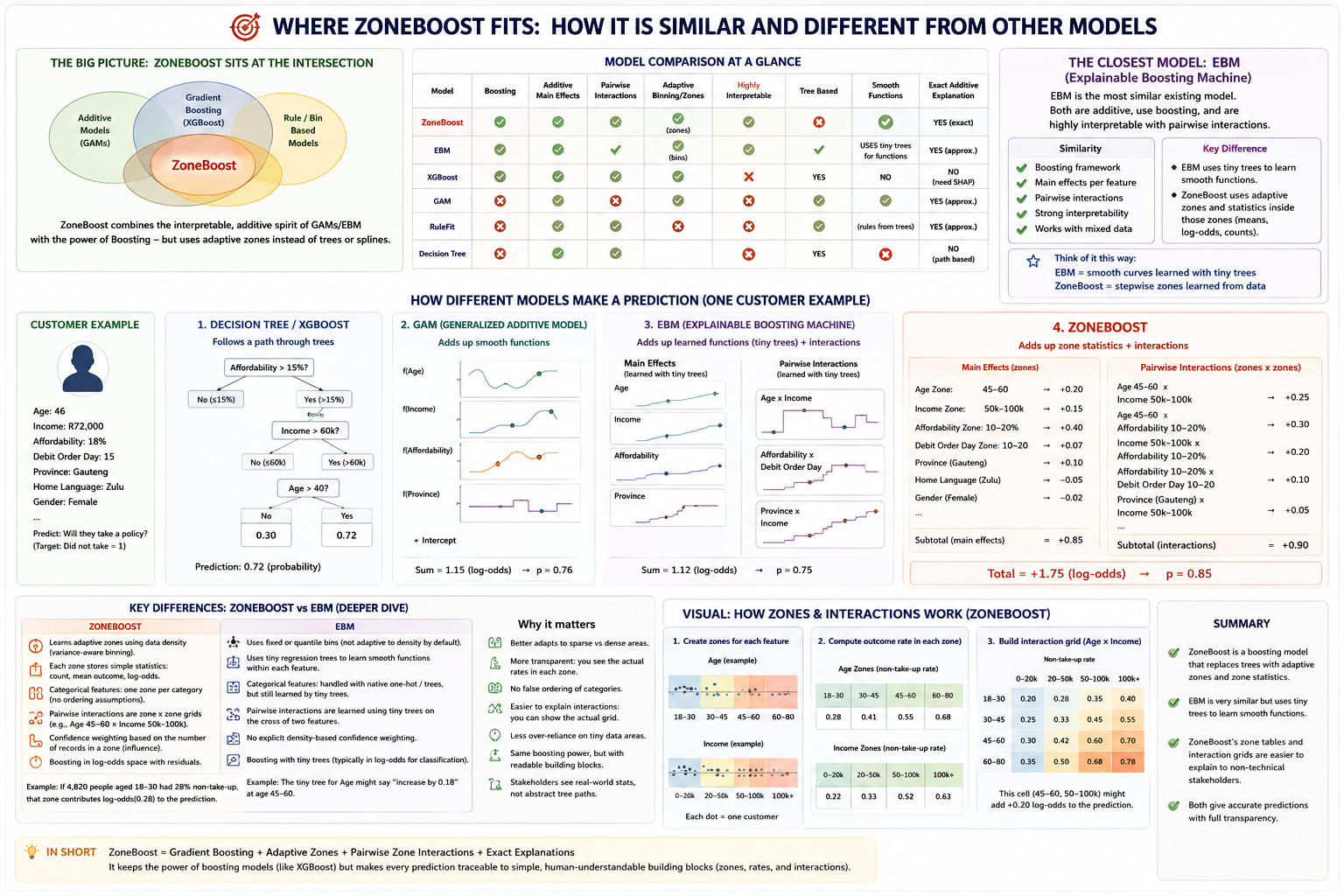
How It Compares
zoneboost sits at the intersection of additive models (GAMs), boosting frameworks (like XGBoost), and rule/bin-based models — combining the interpretable, additive spirit of GAMs and Explainable Boosting Machines (EBM) with the power of boosting, but using adaptive zones and zone-grid statistics instead of trees or splines. EBM is the closest existing model: both are additive, use boosting, and are highly interpretable with pairwise interactions — the difference is that EBM learns smooth functions with tiny regression trees inside each feature, while zoneboost learns adaptive zones and plain descriptive statistics (counts, means, log-odds) inside those zones.